LandComp is a package for quantifying landscape
diversity and structure at multiple scales. For these purposes
Juhász-Nagy’s functions, i.e. compositional diversity (CD) and
associatum (AS), are calculated.
Examples
Suggest we have data on some vegetation types along a landscape. Note, there are three requirements:
- the landscape data should be numeric binary, i.e. it should contain 0 or 1 values
- the geometry of the landscape data should be a regular square or hexagonal grid
- the geometry of the landscape data should have projected coordinates (i.e. WGS84 is not eligible)
Using regular square grid
Have a look at the square grid data.
suppressPackageStartupMessages(library("sf"))
library(LandComp)
data("square_data")
str(square_data)
#> Classes 'sf' and 'data.frame':   300 obs. of  6 variables:
#>  $ VT1     : num  0 0 0 0 0 0 0 0 0 0 ...
#>  $ VT2     : num  0 0 0 0 0 0 0 0 0 0 ...
#>  $ VT3     : num  0 0 0 0 1 1 0 0 0 0 ...
#>  $ VT4     : num  0 0 0 0 0 0 0 1 1 1 ...
#>  $ VT5     : num  0 0 0 0 0 0 0 0 0 1 ...
#>  $ geometry:sfc_POLYGON of length 300; first list element: List of 1
#>   ..$ : num [1:5, 1:2] 400000 400000 405000 405000 400000 ...
#>   ..- attr(*, "class")= chr [1:3] "XY" "POLYGON" "sfg"
#>  - attr(*, "sf_column")= chr "geometry"
#>  - attr(*, "agr")= Factor w/ 3 levels "constant","aggregate",..: NA NA NA NA NA
#>   ..- attr(*, "names")= chr [1:5] "VT1" "VT2" "VT3" "VT4" ...
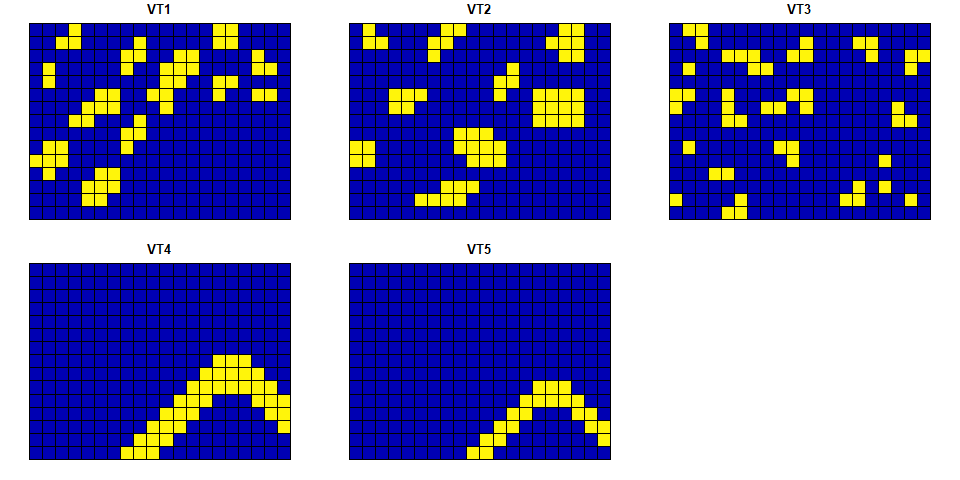
Fig. 1. Visualization of the square grid data.
CD and AS of the landscape at the scale of the base square grid (i.e. using the input grid cells as spatial units) can be calculated as
LandComp(x = square_data, aggregation_steps = 0)
#>   AggregationStep SpatialUnit_Size SpatialUnit_Area SpatialUnit_Count
#> 1               0                1          2.5e+07               300
#>   UniqueCombination_Count   CD_bit    AS_bit
#> 1                      13 2.755349 0.1709469
However, Juhász-Nagy’s functions, i.e. compositional diversity (CD) and associatum (AS) should be calculated at multiple scales. For this purpose spatial units can be selected using a buffer of grid cells around the central grid cell, where 0 means the original cell without enlargement.

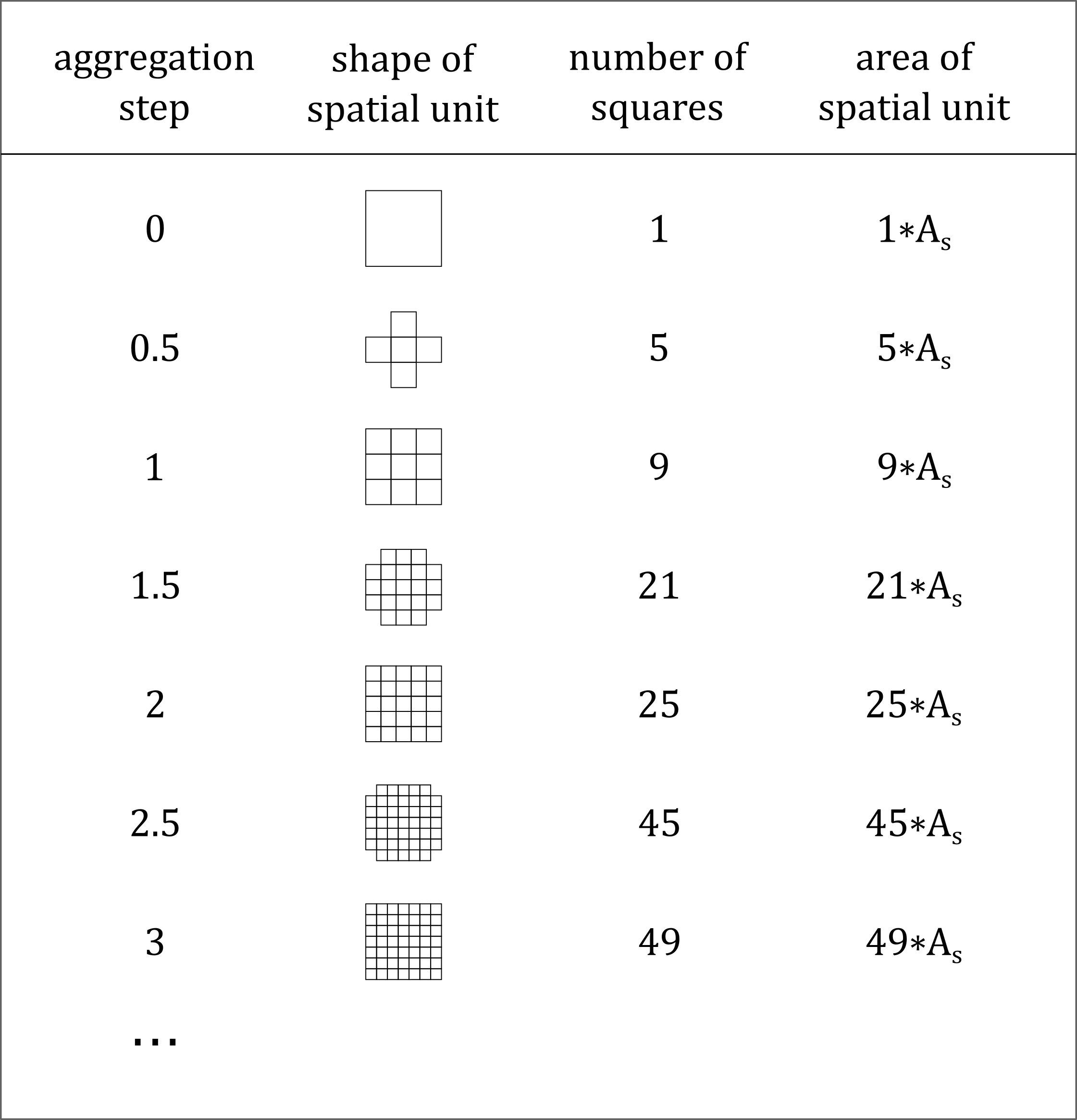
Fig. 2. Main properties of the spatial units used for the calculation of Juhász-Nagy’s functions. In the integer aggregation steps, radially enlarged spatial units consisting of 9, 25, 49 etc. squares are produced. Enlarged spatial units of fraction aggregation steps are created using the spatial unit of the next integer aggregation step, but excluding the grid cells that touch the corners of the next integer unit. As is the area of the square grid cell of the input data.
The analysis can be done more precise by giving also fraction numbers as input. Thus, the following values of CD and AS can be calculated as e.g.
Using regular hexagonal grid
The example dataset contains pointy-topped hexagons. Note, the methods are also fine for regular hexagonal grids containing flat-topped hexagons. Have a look at the hexagonal grid data.
data("hexagonal_data")
str(hexagonal_data)
#> Classes 'sf' and 'data.frame':   300 obs. of  6 variables:
#>  $ VT1     : num  0 0 0 0 0 0 0 0 0 0 ...
#>  $ VT2     : num  0 0 0 0 0 0 0 0 0 0 ...
#>  $ VT3     : num  0 0 0 0 0 0 0 0 0 0 ...
#>  $ VT4     : num  1 1 0 1 1 1 0 1 1 1 ...
#>  $ VT5     : num  0 0 1 1 0 0 1 0 0 1 ...
#>  $ geometry:sfc_POLYGON of length 300; first list element: List of 1
#>   ..$ : num [1:7, 1:2] 649500 649000 649000 649500 650000 ...
#>   ..- attr(*, "class")= chr [1:3] "XY" "POLYGON" "sfg"
#>  - attr(*, "sf_column")= chr "geometry"
#>  - attr(*, "agr")= Factor w/ 3 levels "constant","aggregate",..: NA NA NA NA NA
#>   ..- attr(*, "names")= chr [1:5] "VT1" "VT2" "VT3" "VT4" ...
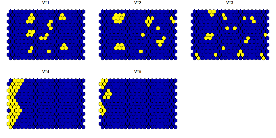
Fig. 3. Visualization of the hexagonal grid data.
CD and AS of the landscape at the scale of the base hexagonal grid (i.e. using the input grid cells as spatial units) can be calculated as
LandComp(x = hexagonal_data, aggregation_steps = 0)
#>   AggregationStep SpatialUnit_Size SpatialUnit_Area SpatialUnit_Count
#> 1               0                1         866025.4               300
#>   UniqueCombination_Count   CD_bit    AS_bit
#> 1                      12 1.972863 0.1256525
However, Juhász-Nagy’s functions, i.e. compositional diversity (CD) and associatum (AS) should be calculated at multiple scales. For this purpose spatial units can be selected using a buffer of grid cells around the central grid cell, where 0 means the original cell without enlargement.

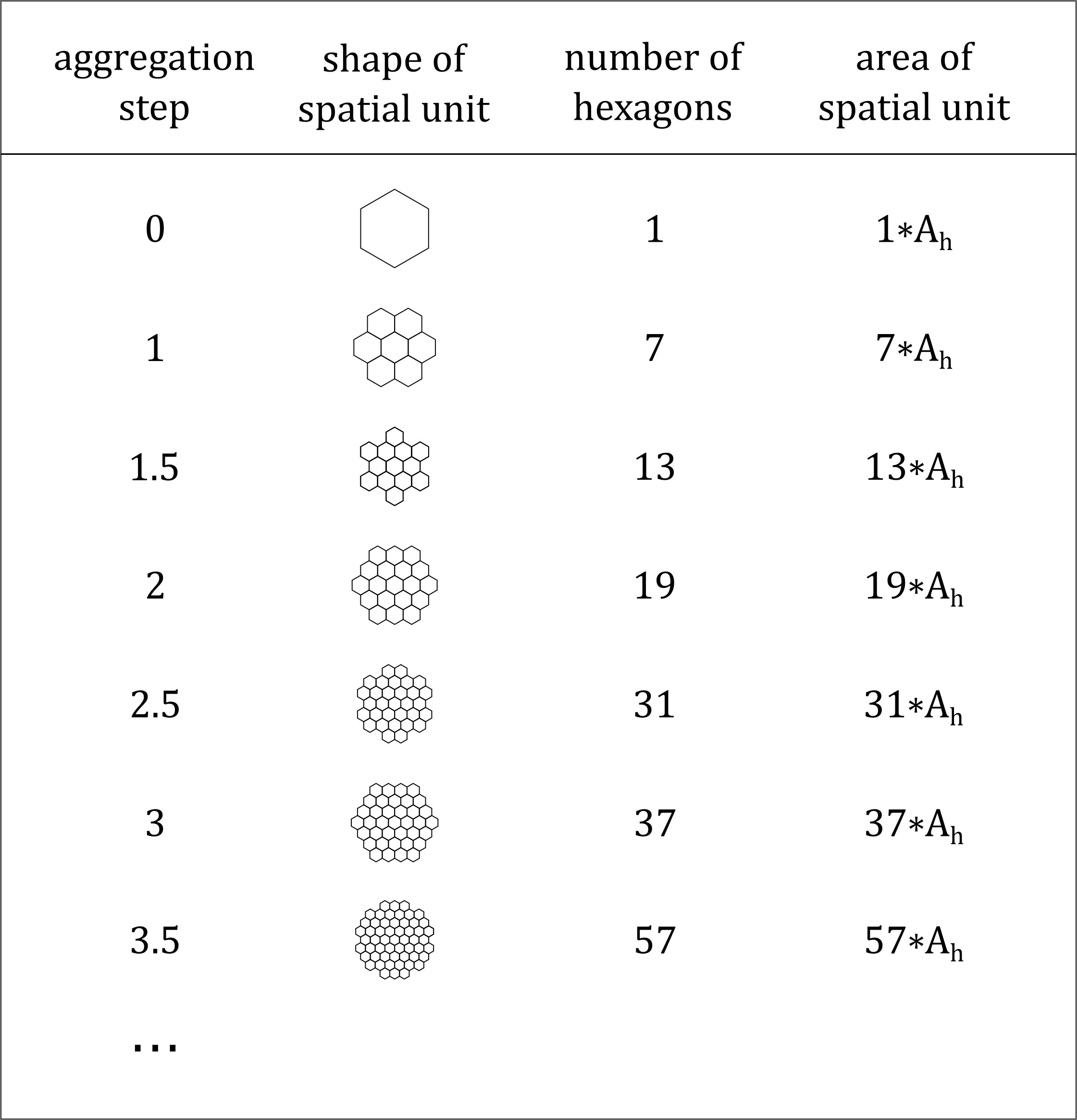
Fig. 4. Main properties of the spatial units used for the calculation of Juhász-Nagy’s functions. In the integer aggregation steps, radially enlarged spatial units consisting of 7, 19, 37 etc. hexagons are produced. Enlarged spatial units of fraction aggregation steps are created using the spatial unit of the next integer aggregation step, but excluding the grid cells that touch the vertices of the next integer unit. Ah is the area of the hexagonal grid cell of the input data.
Analysis can be done more precise by giving also fraction numbers as input. Thus, the following values of CD and AS can be calculated as e.g.
LandComp(x = hexagonal_data, aggregation_steps = c(1, 1.5))
#>   AggregationStep SpatialUnit_Size SpatialUnit_Area SpatialUnit_Count
#> 1             1.0                7          6062178               234
#> 2             1.5               13         11258330               187
#>   UniqueCombination_Count   CD_bit    AS_bit
#> 1                      16 3.422409 0.5394512
#> 2                      21 3.487383 0.5487755
Note, in the case of hexagonal grid, steps falling in the interval ]0,1[ cannot be evaluated.
